Charge flipping in
GSAS-II
Prerequisite:
In this exercise you will use GSAS-II to solve the structure of jadarite (aka “kryptonite”) from powder diffraction data via charge flipping. This structure was originally solved by Pam Whitfield from laboratory powder data in the space group P21/c.
If you have not done so already, start GSAS-II and open the GSAS-II project file (I called it jadarite.gpx) you saved from the second part of the peak fitting-indexing exercise. If you didn’t do that exercise, do it now.
Step 1. Setup for Pawley refinement
There are a number of steps that must be done in preparation for a Pawley refinement after having completed the unit cell indexing and new phase creation. These cover two things: one is to prepare the powder pattern (reset limits, etc.) and the other is to prepare the phase for the refinement.
1. Select Limits in the GSAS-II data tree for the PWDR data set and expand the plot so that the region near d=1.0Å is readily seen. This is ~24deg 2Q. It is an area relatively clear of peaks and makes a good place to end the calculations with a reflection set of ~1Å resolution as needed for charge flipping. Enter 24 for Tmax as the upper limit and make a note of the exact d-spacing (0.9945Å) using the mouse cursor on the plot.
2. Select Instrument Parameters and uncheck all Refine flags and do Operations/Reset profile to recover the default values. The peak fitting done earlier is over a much more limited range of 2Q giving values that will not extrapolate well over the wider range to be used in the Pawley refinement. We will refine them again later.
3. Select Sample Parameters and uncheck refinement of Histogram scale factor.
4. Go to Phases/kryptonite to find the Pawley controls. Check the Do Pawley refinement box and enter the d-spacing (0.9945) into the Pawley dmin box.
5. Also set Pawley neg. wt. to 0.001; this will force all Pawley reflection intensities to be > 0.
When done the General tab should look like

Next find the Data tab; it will be empty except for a single line of text. Do Edit Phase/Add powder histograms; a dialog box will appear

Select the one possibility; the desired data set will be added to this phase for analysis. The data tab now shows the new data set; check the Show button to see the full information

I’ve stretched the window slightly to see the entire contents. This is the location for all the phase dependent parameters for this histogram. Notice that it includes phase fraction, size & mustrain as well as preferred orientation, elastic strain and extinction corrections. The Babinet correction is intended for protein work where a significant region of the structure is disordered solvent. There are buttons for plotting size and mustrain surfaces and preferred orientation correction curves.
Next find the Pawley reflections tab; it will be empty except for column headings. Do Operations/Pawley create; this makes the reflection set over the range covered by setting Pawley dmin. The table should list reflections 0-629. Select and check the refine column using the same technique you used for the peak list.

This completes the Pawley refinement setup; be careful that you didn’t skip a step as it might not work correctly if you did.
Step 2 Pawley refinement
To start the refinement, do Calculate/Refine on the main GSAS-II data tree window. Before it begins a backup of the project file is made; the name will be jadarite.bck0.gpx. It can be used to recover from a bad refinement. A progress dialog box will appear showing the residual as the refinement proceeds. My refinement completed with Rwp ~15.0%; a dialog box appears asking if you wish to load the result. Press OK. To see the plot select the PWDR line in the GSAS-II data tree (I’ve adjusted the width and height).
It is evident from examining the plot that improvement can be had by refining the lattice parameters. Go to Phases/kryptonite in the GSAS-II data tree and check the Refine unit cell box. Repeat Calculate/Refine. I obtained a new residual of 10.36%.
Now select Instrument parameters for the PWDR data set in the GSAS-II data tree and check U, V, W, X & Y. Repeat Calculate/Refine; I obtained an improved residual of 9.7% with a much better fit at the high angle part of the pattern.
This may be good enough to try charge flipping.
Step 3 Charge flipping
A few steps are needed to set up for a charge flipping run. Go to Phases/kryptonite and notice the Charge flip controls in the middle of the General tab.
1. Select Reflection set from to be PWDR 11bmb_6231.fxye Bank 1 (the only choice!). This makes the reflection set to be used those in Reflection Lists under the PWDR data set; these should match the Pawley reflection set.
2. Set the Peak cutoff (in Fourier map controls) to 10%. This controls the map search routine.
For powder data it is not usually advisable to select a Normalizing element; if selected a periodic table appears – select an element or ‘None’. The Resolution defines the map spacing and thus the extent of the reflection set; the observed reflection set is zero filled to this limit for charge flipping. The k-factor and k-Max determine the lower threshold and upper limit for charge flipping, respectively. The latter is used to avoid “Uranium solutions” in the result. Set this to 10-12 for equal atom problems and larger for heavy atom ones. The default (20) is suitable for kryptonite.
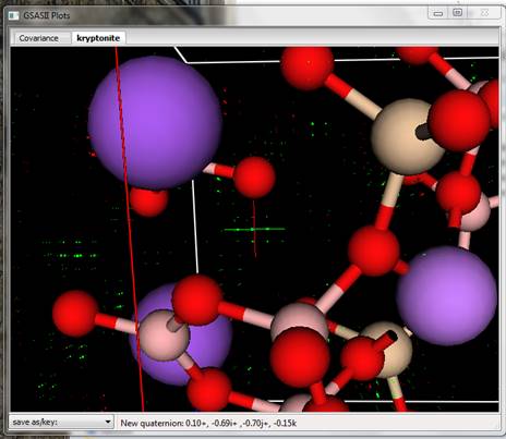
When ready select Compute/Charge flipping; a progress bar dialog will appear that tracks the residual found in each charge flipping cycle. It will quickly drop to some level and then perhaps drop again into the 20-30% range for a successful charge flipping run. Press Cancel to stop the charge flipping; a peak list and a drawing of the solution will appear. One of my runs gave

The result looks very promising! Charge flipping operates without regard to symmetry and GSAS-II attempts to locate the map with respect to the symmetry elements from the computed reflection phases. Errors in these phases can disrupt this process so that the map and peak positions are offset from their true positions. To discover this and fix it, rotate the drawing around to check that atom positions are related via the inversion center (the multicolored cross in the center of the cell. NB: only works if structure has an inversion center!). Avoid motions with the right mouse button pressed, this moves the cross. To recover, press the ‘C’ key to reset the cross to the cell center. If you find an offset to the map, orient it so the offset is horizontal or vertical and then press the L, R, U or D keys to shift the map and peaks as needed. The shift is in resolution units (0.5Å) so the fix can only be approximate. Repeat as needed. Notice that the peak positions in the table are updated as the offset is changed. In this case, I needed just a single step to correct the map offset. NB: you can use these keys to move the result anywhere you wish, e.g. to select a different origin for the structure but pay attention to the location of symmetry elements.
Step 4 Obtain solution from charge flip result
The next step is to extract the unique peak positions from the map and make atoms out of them. The map peak list is sorted with the highest peak first; you can change the sorting to be along any of the column headings in the table by a single click on the desired heading. The dzero column gives the distance of each peak from the origin. The menu items under Map peaks give you several tools to aid in the peak selection process, we will just use a couple in this example. I have chosen to proceed by sorting the atoms by dzero, selecting all and then finding the unique ones.
1. Do a single click on the dzero column heading. This will sort the peaks in increasing distance from the origin.
2. Do a single click on the upper left (empty) box of the table. All entries will be colored grey indicating their selection.
3. Do Map peaks/Unique peaks. That should select (grey) 13-14 out of 52 peak positions in the table and all should be near the top of the list. They will be colored green in the plot. If more are selected then check the map offset – it may need a slight correction.
These are now ready to turn into atoms. Do Map peaks/Move peaks. The drawing will show white balls for each of the selected positions and the Atoms table will now have 13 new H atoms. We are looking for heavier atoms in the formula NaSiO8B3LiH so 13 atoms should correspond to all but the Li & H atoms.

The atom names indicate the peak magnitude to aid identification (M100 for the largest in the Map peaks table which may not be one of those moved to the Atoms table). You can hand sort them by selecting a row with the Alt key (or Shift/Ctrl keys) down and then selecting a position in the table with the Alt key still down. On Linux machines the Alt key may have been hijacked by the operating system; use Shift/Ctrl instead to move atoms. My list is now
Do an Edit/Reload draw atoms from the Atoms menu to make the drawing reflect the change in atom ordering. Go to Draw Atoms and double click the upper left box (empty); the entire table will be selected (gray). Then do Edit Figure/Fill Unit Cell; the structure will be redrawn with all the equivalent positions shown.

To proceed, one could select an atom and see its bonding pattern with its neighbors to identify it. Then pick its neighbors and identify them continuing on until all atoms are identified. In my case this would be:
1. Go to the Atoms tab and pick M83; it is bonded to 4 neighbors (two are in next cell) as a tetrahedron. Probably Si. Change its Type. The plot will change the green (as selected) ball to a gold colored one (the color assigned to Si). You may have to rock the structure slightly to make the change happen. The equivalent ones are also shown; some show the four neighbors as a tetrahedron.
2. Pick its neighbors and change them to O atoms. A shift left mouse button on each will select them. The atoms will change from green to red.
3. Pick an O-atom neighbor; it will be a B-atom.
4. And so on until each atom is identified. NB: the Na & Li (if seen) atoms will be relatively isolated.
When I finished my structure looked like
The original charge flipping solution is still visible and the atoms are now identified.
Interestingly the atoms identified exactly matched with the magnitudes of the charge flip map peaks with Si & Na near the top and B at the bottom.
Now one can safely remove the map peaks (do Map peaks/Clear peaks in the Map peaks tab) and clear the charge flip map (do Clear map in the General tab). After dressing up the drawing by making the Na atom van der Waals spheres and the rest as balls and sticks I have a nice drawing of the structure (without the Li and H atoms though).

Save the project file; the next step is to complete the structure by finding the Li and H atoms and then doing the Rietveld refinement on the completed structure.
Step 5 Complete the structure
To complete the structure you will need to perform a preliminary Rietveld refinement. This will make the atom positions more accurate and prepare a set of calculated structure factors needed to generate a difference Fourier map good enough to reveal the Li atom position and maybe the H-atom as well. There are a number of steps needed to set all the controls from the previous Pawley refinement to get a successful start for the Rietveld refinement.
1. Go to the Instrument Parameters entry in the GSAS-II data tree and uncheck all Refine boxes. You don’t want to start with these when the scale factor is unknown.
2. Go to Sample Parameters and check the Histogram scale factor box. This is the scale factor for the data set. You may want to change the Goniometer radius to 1000. That will put the Sample X displacement on a proper scale when you refine it later.
3. Go to Phases/kryptonite General tab and uncheck Refine unit cell and Do Pawley refinement boxes. The latter is most important; if you forget you will just get another Pawley refinement!
Now do Calculate/Refine from the main GSAS-II data tree menu; all that was refined is scale and background. I got a Rwp ~31%. The plot shows clear intensity differences; the atom positions obviously need refinement.
I’ve shifted & zoomed in to make the differences more obvious.
Go to Phases/kryptonite and select the Atoms tab. The double click the refine column heading, a dialog box will appear, select the X-coordinates box and press OK. The atoms table will show the refinement controls
Do Calculate/Refine again; my Rwp is now ~15%. You can now safely refine lattice
parameters (in the General tab for Phases/kryptonite)
and the Instrument
parameters U, V, W,
X & Y.
My refinement improved slightly to Rwp~14.5%. Let’s see if a difference Fourier
map will show anything.
Go to the Phases/kryptonite
General tab; the Fourier map controls are midway
down the window.
1. Select delt-F for the Map type.
2. Select PWDR 11bmb_6231.fxye Bank 1 for the Reflection set from item (the only choice). The Fourier calculation will use the structure factors shown in the Reflection list item for this PWDR data set.
3. Do Compute/Fourier map from the General tab window. The map will be computed via fast Fourier techniques and is very fast. A few lines summarizing the map is printed on the console, the structure plot may show a single green dot somewhere (it could be hidden beneath an atom!), this is the highest point in the map.
4. Go to the Draw Options tab and adjust the Contour level slider until something appears on the map.

What is drawn here are green dots whose size are proportional to the electron density. These are the Li atom positions. There are several ways within GSAS-II to add it to the atom list. One is to do Compute/Search map in the General tab and then find them in the Map peaks tab much the same way we did earlier in this exercise. Another is to get the atom position directly from the map, we will do that now.
1. Go to the Phases/kryptonite Atoms tab.
2. Using the mouse, position the multicolored cross directly in the center of one of the presumed Li atom peaks. Rotate the drawing around with the left mouse button and shift the cross with the right mouse button. You can zoom in using the roll wheel on the mouse (or else use the Camera distance slider in the Draw Options tab if your mouse lacks a wheel).
3. Do Edit Atoms/Insert view point, a white ball will appear at the selected position and an H-atom (name = UNK) will be appended to the end of the atom list.
4. Change its Type to Li, it will be renamed and the ball color/size will change to that for Li.


Change the refine flag to X for the Li atom and repeat Calculate/Refine from the main GSAS-II data tree window. My residual Rwp dropped to ~11.3%. Next set all refine flags to XU and repeat Calculate/Refine. My residual is now Rwp ~10.8%. Maybe we can find the H-atom.
From the General tab, Do Compute/Fourier map and adjust the Contour level in the Draw options tab.
I moved the cross to a very interesting feature of the map and zoomed in a bit. This may be the H-atom, Insert view point from the Atoms tab and change the Type to H (I know it is H already but this step changes the name from UNK). Repeat the Calculate/Refine without varying any of the H-atom parameters; my final Rwp = 10.69% (you don’t get much improvement for adding an H-atom to an oxide structure).